A Multiscale Numerical Study of Hurricane Andrew (1992). Part IV: Unbalanced Flows
Zhang, D.-L., Y. Liu and M.K. Yau
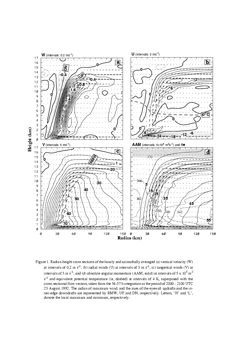
Figure 1. Radius-height cross sections of the hourly and azimuthally averaged (a) vertical velocity (W) at intervals of 0.2 m s-1; (b) radial winds (U) at intervals of 3 m s-1; (c) tangential winds (V) at intervals of 5 m s-1; and (d) absolute angular momentum (AAM, solid) at intervals of 5 x 10⁵ m2 s-1 and equivalent potential temperature (q e, dashed) at intervals of 4 K, superposed with the cross-sectional flow vectors, taken from the 56-57 h integration or the period of 2000 - 2100 UTC 23 August 1992. The radius of maximum wind, and the axes of the eyewall updrafts and the inner-edge downdrafts are represented by RMW, UP and DN, respectively.
Figure 2. As in Fig.1 but for the AAM budget: (a) the net Lagrangian tendency due to all the sources/sinks (dM/dt); (b) the horizontal advection (MH); (c) the vertical advection (MV); and (d) the local tendency (Mt). (a) and (d) are contoured at ± 0.5, ± 1, ± 2.5, ± 5, ± 10, ± 20, and ± 30 x 105 m2 s-1 h-1, while (b) and (c) are contoured at ± 2.5, ± 5, ± 10, ± 20, ± 30, and ± 40 x 105 m2 s-1 h-1.
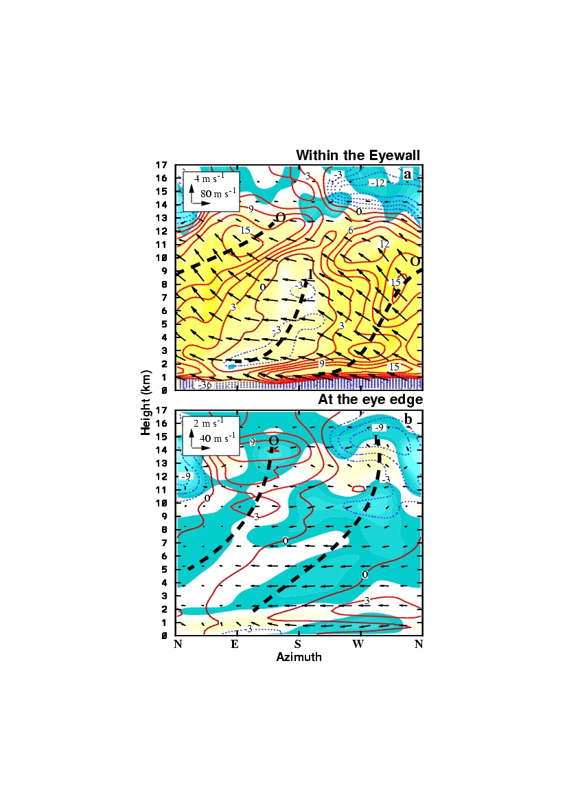
Figure 3. The azimuth-height cross sections of the temporally-averaged system-relative radial flow (every 3 m s-1) with the downdrafts shaded that are taken along the slanting surfaces (a) in the eyewall (i.e., from R = 30 km at the surface to R = 70 km at the 17-km height), and (b) in the eye (i.e., from R = 5 km at the surface to R = 70 km at the 17-km height) from the 56-57 h integration. The right axes show the radius in km at a few selected heights. Thick dashed lines denote the axes of incoming (I) and outgoing (O) air. Solid (dashed) lines are for positive (negative) values. In-plane flow vectors are superposed.
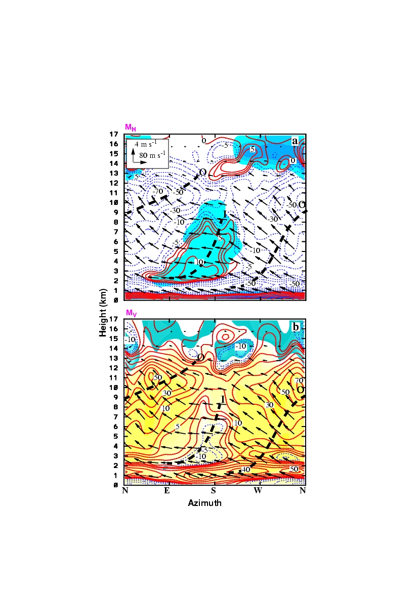
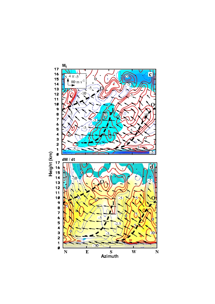
Figure 4. As in Fig. 3a but for the AAM budget in the eyewall: (a) horizontal advection (MH) with the inflow shaded; (b) vertical advection (MV) with the downdraft shaded; (c) local tendency (Mt) with the inflow shaded; and (d) Lagrangian tendency (dM/dt), contoured at 0, ± 2.5, ± 5, ± 10, ± 20, ± 30, ± 40, and ± 50 x 105 m2 s-1 h-1.
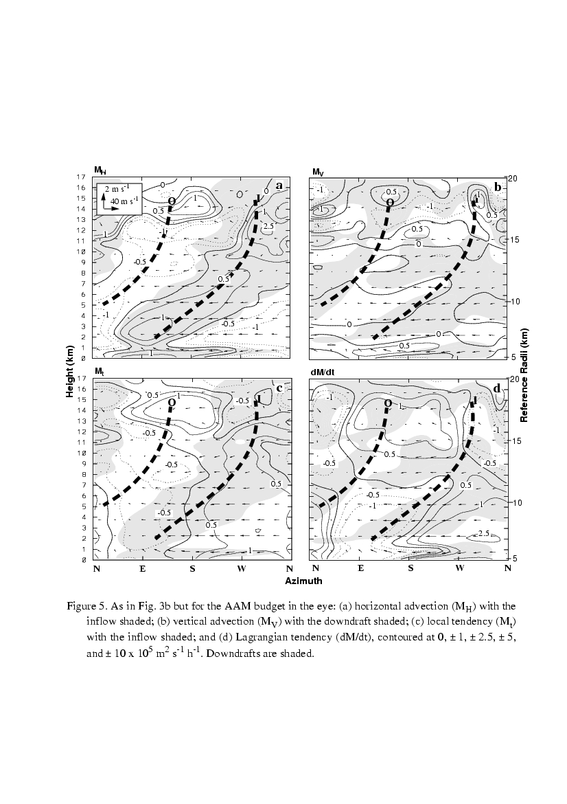
Figure 5. As in Fig. 3b but for the AAM budget in the eye: (a) horizontal advection (MH); (b) vertical advection (MV); (c) local tendency (Mt); and (d) Lagrangian tendency (dM/dt), contoured at 0, ± 1, ± 2.5, ± 5, and ± 10 x 105 m2 s-1 h-1. Radial inflows are shaded in (a) and (c), and downdrafts are shaded in (b) and (d).
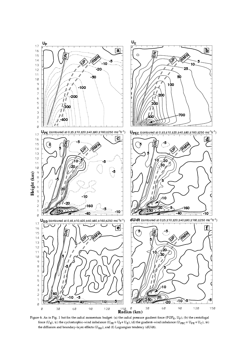
Figure 6. As in Fig. 1 but for the radial momentum budget (unit: m s-1 h-1 ): (a) the radial pressure gradient force (PGFR, UP); (b) the centrifugal force (UE); (c) the cyclostrophic-force imbalance (UPE = UP+ UE); (d) the gradient-force imbalance (UPEC = UPE + UC); (e) the diffusion and boundary-layer effects (UB); and (f) Lagrangian tendency (dU/dt).
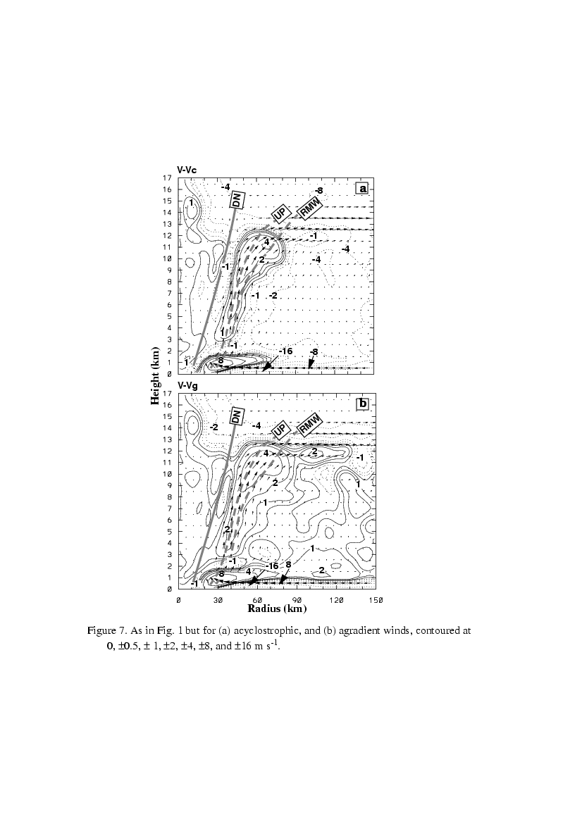
Figure 7. As in Fig. 1 but for (a) acyclostrophic winds (V - VC); and (b) agradient winds (V - Vg), contoured at 0, ± 0.5, ± 1, ± 2, ± 4, ± 8, and ± 16 m s-1. In-plane full flow vectors are superposed.
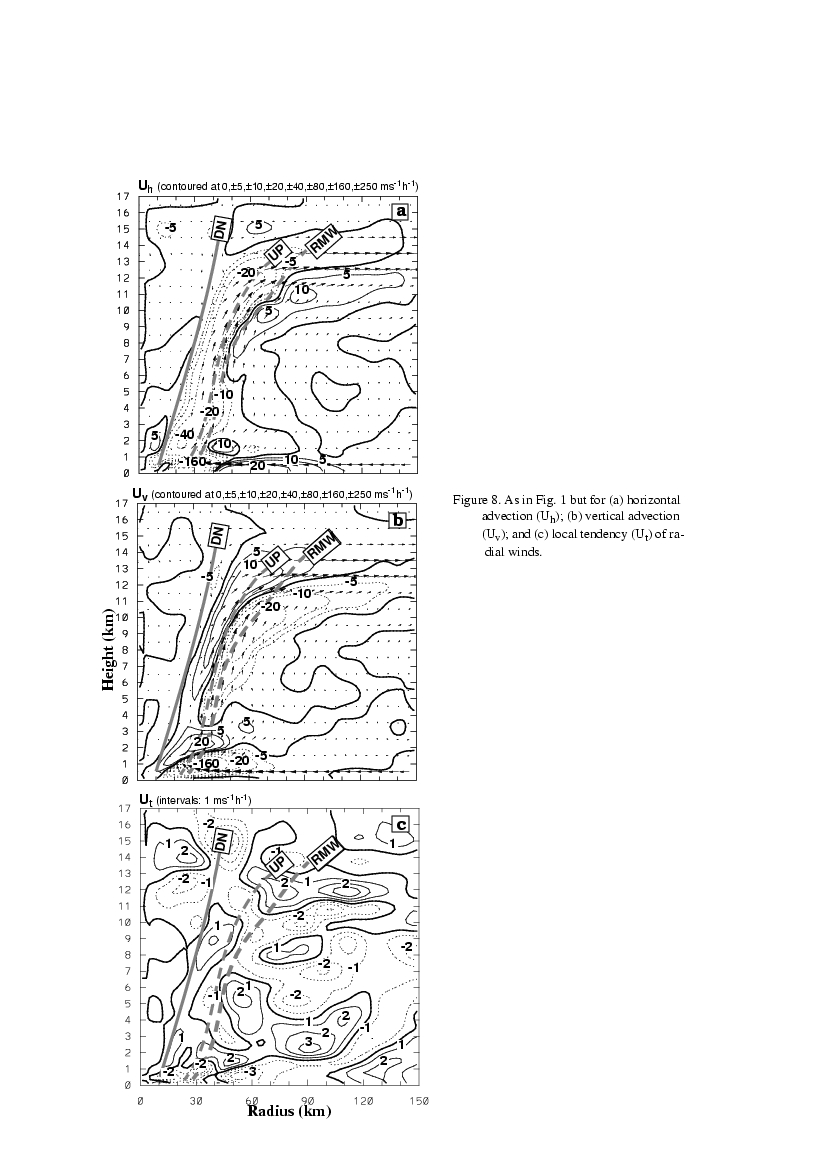
Figure 8. As in Fig. 1 but for (a) horizontal advection (UH); (b) vertical advection (UV); and (c) local tendency (Ut) of radial momentum.
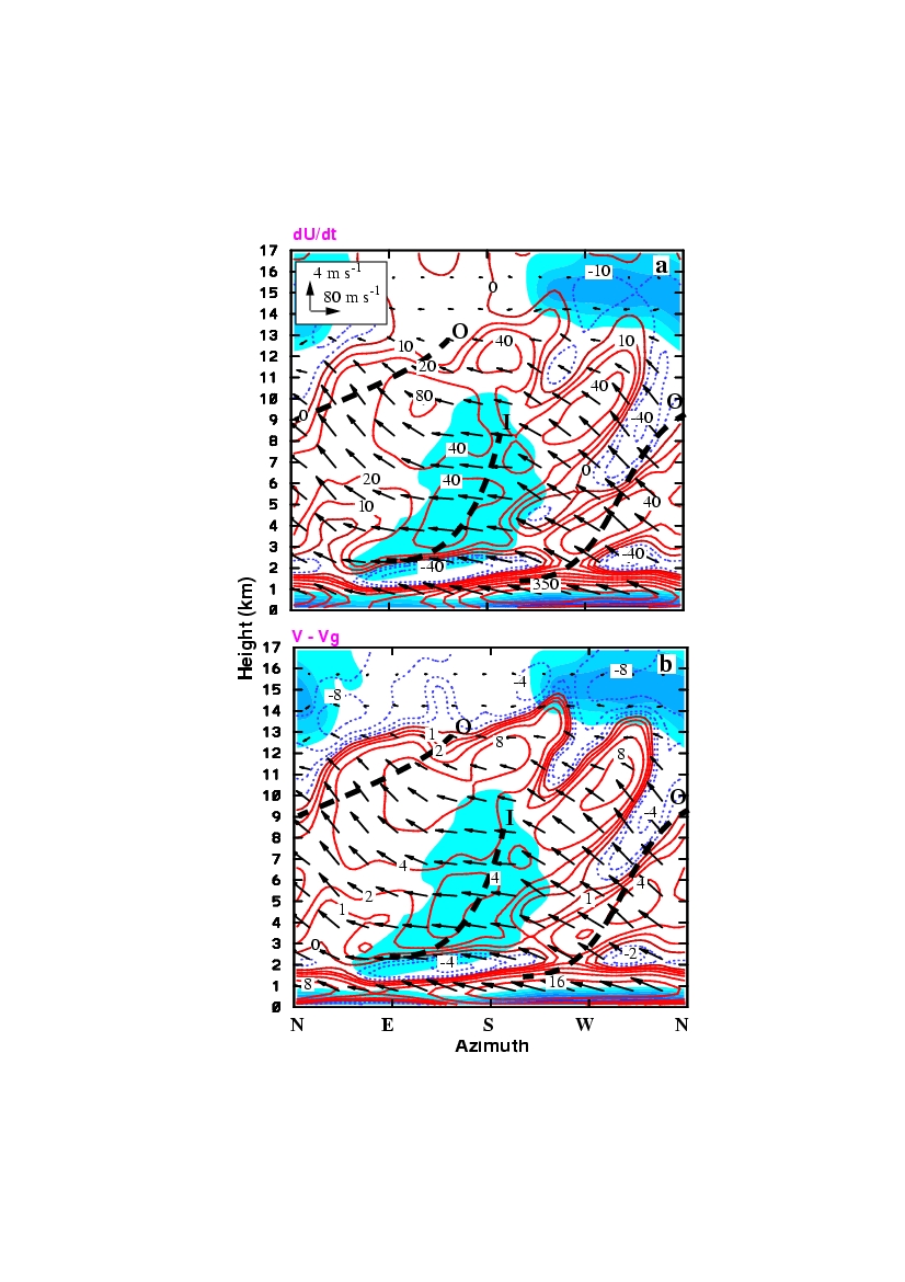
Figure 9. As in Fig. 3a but for (a) the Lagrangian radial momentum tendency (dU/dt), contoured at 0, ± 10, ± 20, ± 40, ± 80, ± 160, ± 320 and ± 350 m s-1 h-1 ; and (b) agradient winds (V - Vg), contoured at 0, ± 1, ± 2, ± 4, ± 8, and ± 16 m s-1. The inflow regions are shaded.
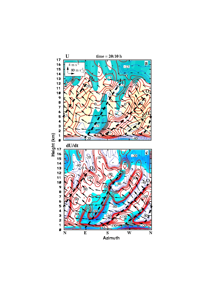
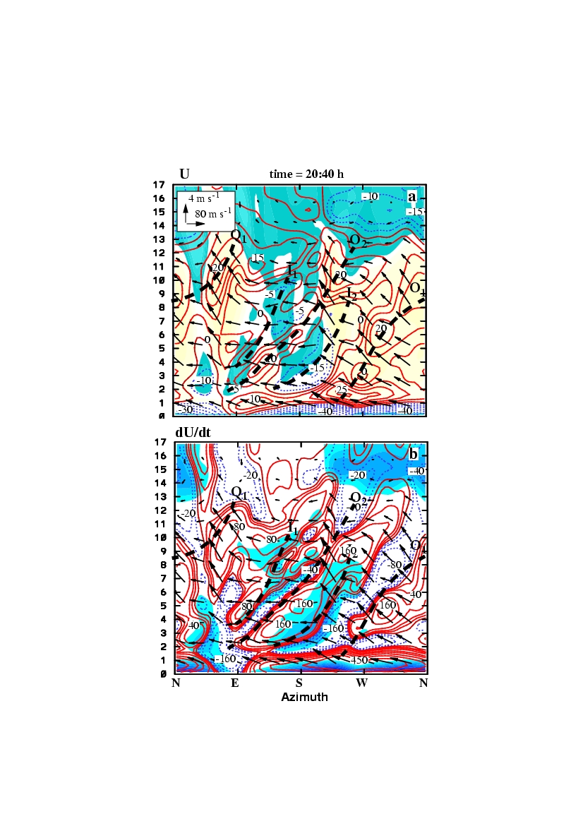
Figure 10. As in Fig. 3a but for the instantaneous fields in the eyewall: (a) and (b): (a) the system-relative radial flow (every 3 m s-1) with the downdrafts shaded; (b) the Lagrangian radial momentum tendency (dU/dt), contoured at 0, ± 10, ± 20, ± 40, ± 80, ± 160, and ± 320 m s-1 h-1 , with the inflow shaded. They are taken from the simulation valid at 2010 UTC 23 August 1992. (c) and (d) As in (a) and (b) but for 2040 UTC 23 August 1992.
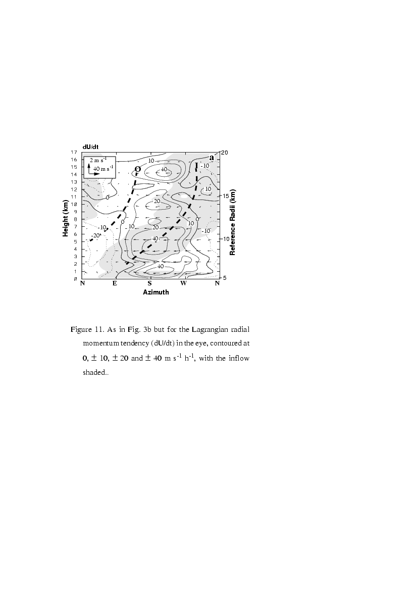
Figure 11. As in Fig. 3b but for the Lagrangian radial momentum tendency (dU/dt) in the eye, contoured at 0, ± 10, ± 20, and ± 40 m s-1 h-1, with the inflow shaded.