1st REOF 1st REOF 1st REOF

(as seen by three data sets)
Data. Monthly sea surface temperatures (SSTs) for this analysis were taken from three data sets. The first one is based on a merged product from HadISST plus OIv2 produced at NCAR (1949-2002); the second data set is the Hadley sea ice and SSTs from the Hadley Centre for Climate (1871-1999, version 1.1), and the final data set is the DaSilva data set from the University of Wisconsin-Milwaukee (1945-1993). Except by the DaSilva data set that is on a 6x2 grid, the other two data sets are on a 1x1 grid. Experiments with the HadISST+OIv2 data set on the 6x2 grid show not a significant impact on the results shown here.
Methodology. Before doing anything, anomalies are calculated with respect to the monthly means (i.e. annual cycle removed), and then an area weighting of the anomalies is done in order to avoid bias due to unequal areas of a latitude-longitude grid. Finaly, the weighted anomalies are normalized dividing them by the square root of the spatially integrated temporal variance. Modes of SST variability are extracted from a covariance-based Rotated Principal Component Analysis of monthly SST anomalies for the mostly Pacific domain (120E-60W,20S-60N) spanning the comon period 1950-1993. EOFs of the covariance matrix are obtained from the Singular Value Decomposition analysis. The eigenvectors are then rotated using the VARIMAX technique.
Results. In
this case 9 eigenvectors were rotated. The explained variance for those
9 eigenvectors is 62.7% for the HadISST+OIv2 data set, 65.9% for the Hadley
data set, and 49.8% for the daSilva data set. theThe first five modes
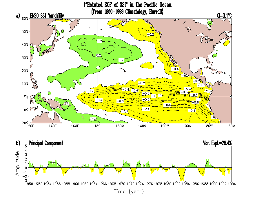
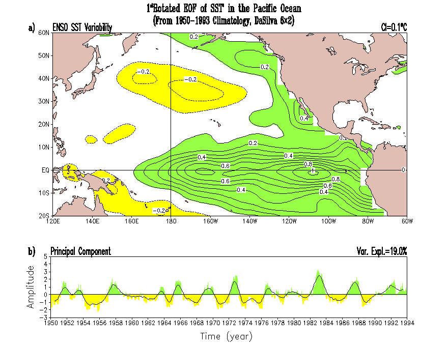
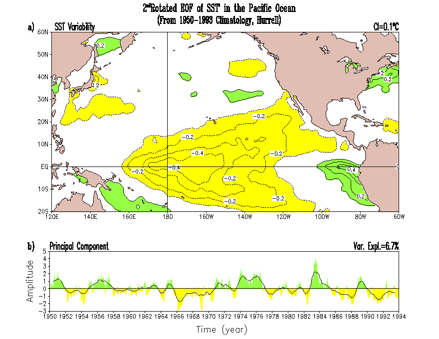
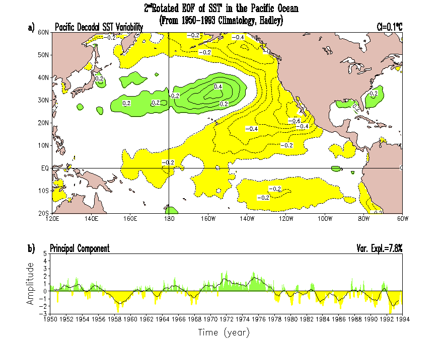
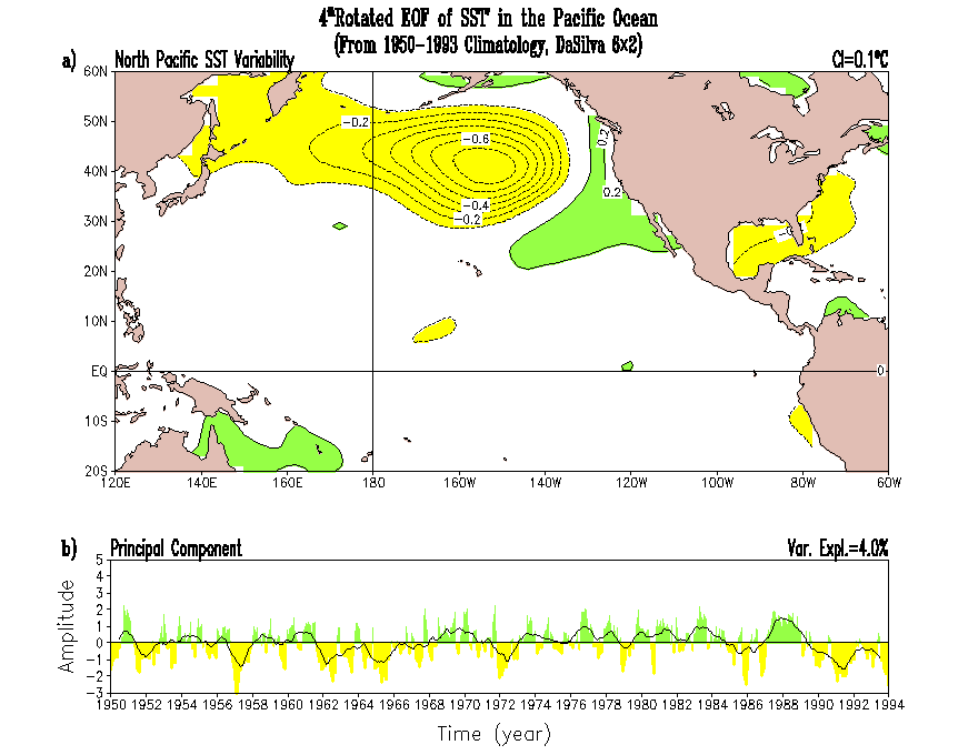
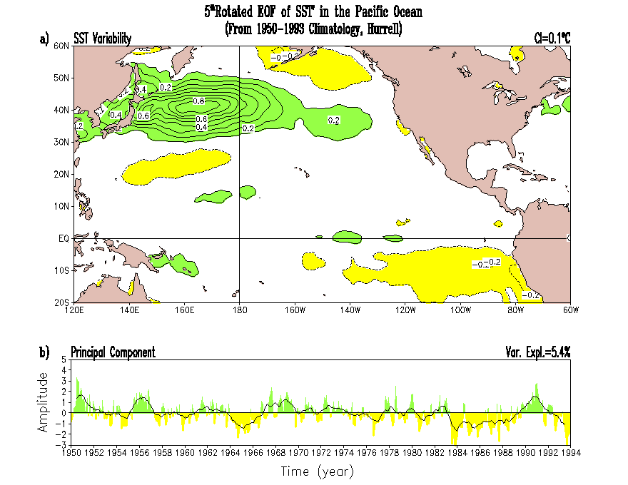
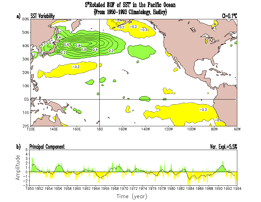
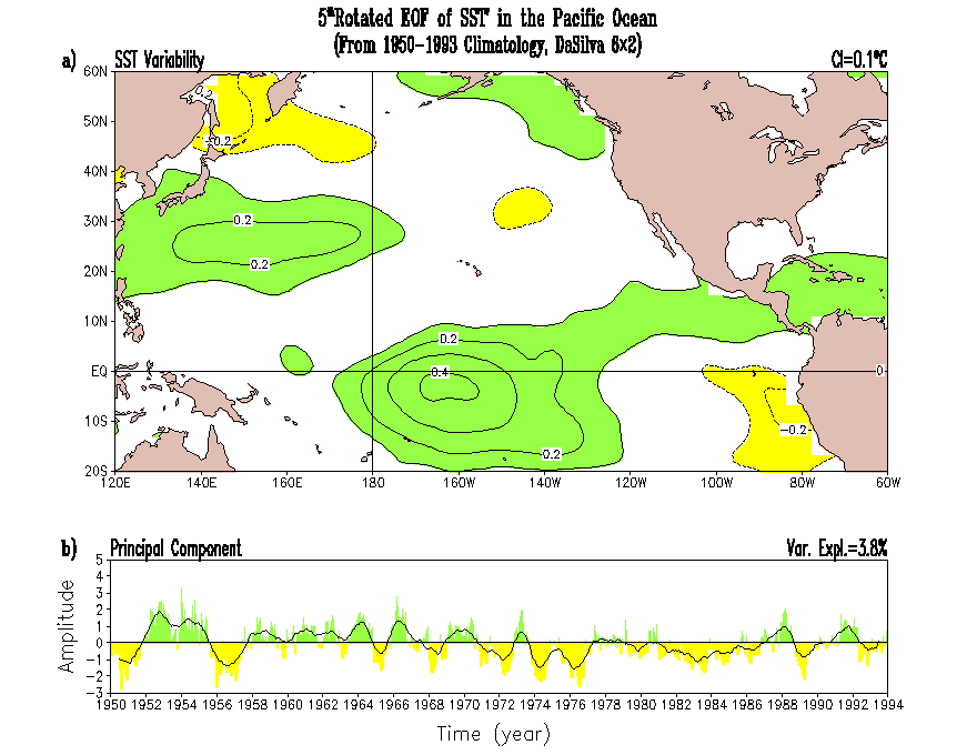
are displayed in the following figures where green/yellow anomalies represent
positive/negative values; time series associated to the modes are also
displayed with a 12-month running mean superimposed to the monthly variation.
HadISST+OIv2 HadleyISST1.1 DaSilva
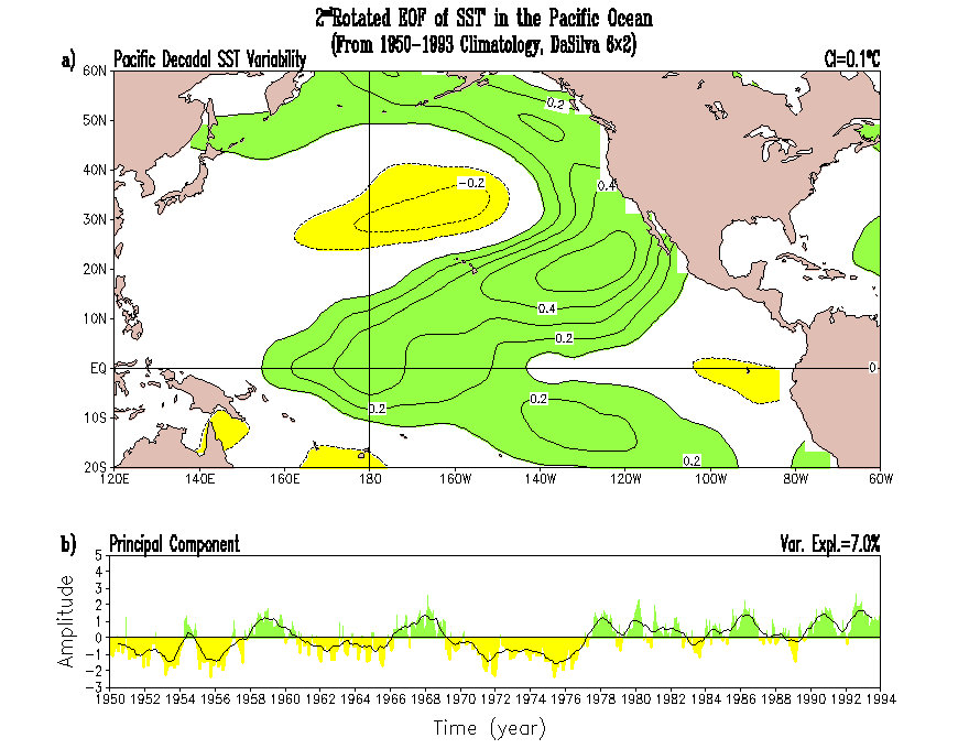
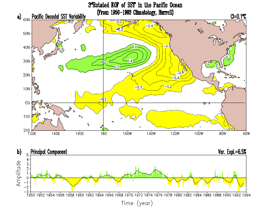
From this analysis is possible to
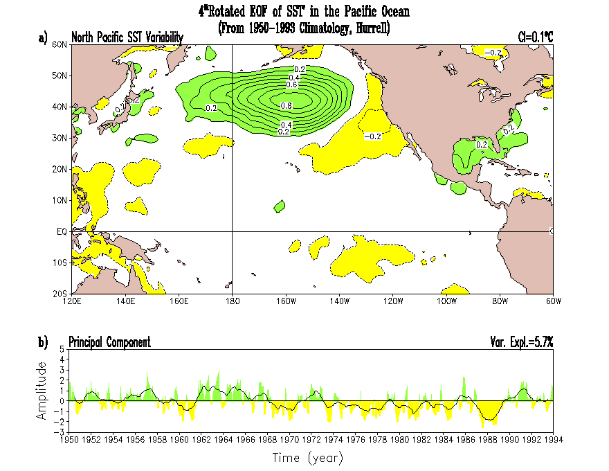
identify five different patterns of anomalies, 1) ENSO, 2) Pacific Decadal
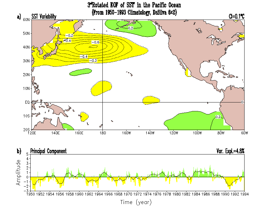
(PDe), 3) North Pacific (NP), 4) Western North Pacific (because anomalies
are concentrated to the western part of the North Pacific -WNP), and 5)
Equatorial "less-than-shape" (with the apex of the shape in the central
Pacific and extending toward both sides of the equator, reaching
the Mexican coasts in the north). An interesting thing to note is that
the order of the modes in the DaSilva data set is not the same as that
shown by Barlow et al. (2001), however, that order of modes is reproduced
when the 1945-1993 period is considered. Another important thing to note
is the fact that the first mode in all the data sets is that corresponding
to ENSO, however, the explained variance is above 26% in the data sets
using HadISST while it is 19% in the DaSilva data set. The order of the
modes is given in the following table.
| MODE | HadISST+OIv2 | HadISST | DaSilva |
| ENSO | 1st: 26.4% | 1st: 27.3% | 1st: 19.0% |
| Pacific Decadal (PDe) | 3rd: 6.5% | 2nd: 7.8% | 2nd: 7.0% |
| North Pacific (NP) | 4th: 5.7% | 4th: 5.8% | 4th: 4.0% |
| Western North Pacific (WNP) | 5th: 5.4% | 5th: 5.5% | 3rd: 4.8% |
| Equatorial
"less-than-shape" |
2nd: 6.7% | 3rd: 6.8% | 5th: 3.8% |
It is clear that the relative importance
of the WNP and Equatorial "less-than-shape" patterns rest weight to the
PDe and NP patterns in the whole analysis. Some questions to answer are
about the high explained variance for the ENSO mode in the data sets using
HadISST, and the increase in explained variance of the ED in those data
sets.

